Introduction to clonal embeddings#

In this notebook, we’re going to build a clonal embedding for the dataset with in vitro hematopoiesis.

[1]:

import scanpy as sc
import numpy as np
import pandas as pd
import seaborn as sns
import matplotlib.pyplot as plt
import clone2vec as c2v

sc.set_figure_params(dpi=80)
sc.settings.verbosity = 3
sns.set_style("ticks")

Preprocessing#

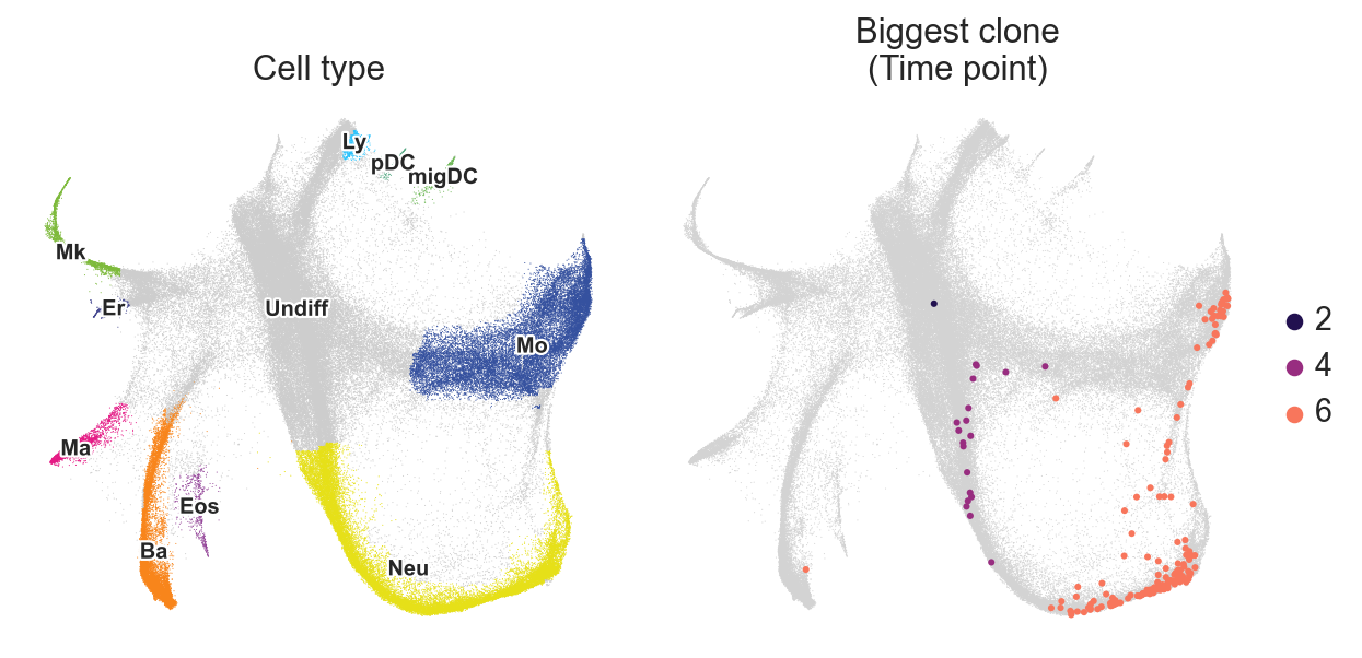
Firstly, let’s take a look at the dataset.

[2]:

adata = c2v.datasets.Weinreb_in_vitro()

[3]:

fig, axes = plt.subplots(ncols=2, figsize=(8, 4))

sc.pl.embedding(
    adata,
    basis="X_spring",
    color="Cell type annotation short",
    frameon=False,
    title="Cell type",
    legend_loc="on data",
    legend_fontsize=9,
    legend_fontoutline=2,
    ax=axes[0],
    show=False,
)

# This function makes possible to plot subparts of the embedding
# on top of the whole embedding
c2v.pl.group_scatter(
    adata,
    groupby="Clone",
    groups=adata.obs["Clone"].value_counts().index[1],
    basis="X_spring",
    title="Biggest clone",
    kwargs_group={"color": "Time point"},
    ax=axes[1],
)

fig.tight_layout()

Secondly, let’s create an AnnData-object with clones instead of cells. In the original dataset, clones from different timepoints and wells are concatenated together. Let’s demultiplex them into days / different wells.

[4]:

adata.obs["time:well:clone"] = (
    adata.obs["Time point"].astype(str) + ":" +
    adata.obs["Well"].astype(str) + ":" +
    adata.obs["Clone"].astype(str)
)

adata.obs["time:well:clone"] = [
    i if not i.endswith(":NA") else "NA"
    for i in adata.obs["time:well:clone"]
]

clones = c2v.pp.clones_adata(
    adata,
    obs_name="time:well:clone",
    min_size=2,
    na_value="NA",
    fill_obs="Cell type annotation short",
)

creating clone-level AnnData
    selected 8173 clones (>= 2)
    finished (0:00:00): created clones AnnData with
     .X float matrix of proportions (clones × categories)
     .layers['proportions'] float matrix with fate proportions
     .layers['counts'] integer matrix with fate counts
     .obs['n_cells'] integer vector with number of cells per clone
     .obs['n_fates'] integer vector with number of fates per clone
     .var['n_clones'] integer vector with number of clones per fate
     .uns['fill_obs'] string label

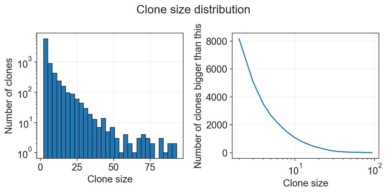
Now we have AnnData object with clones. We can plot amount of cells per clone or amount of fates per clone, and filter based on this values.

[5]:

c2v.pl.clone_size(clones)

We can additionally transfer annotation of clones from cells’ AnnData object.

[6]:

c2v.pp.transfer_annotation(adata, clones, annotation_obs_adata=["Time point", "Well", "Clone"])

transferring annotations between cell and clone objects
    finished (0:00:00): added to clonal AnnData
     .obs['gex_Time point'] categorical labels
     .obs['gex_Well'] categorical labels
     .obs['gex_Clone'] categorical labels

Clonal embedding#

clone2vec is essentially a Skip-Gram algorithm used in the gene expression space instead of bags of words. It might be convenient to think about Skip-Gram as of an Exponential Family PCA (EPCA, or GLM-PCA) of the matrix of counts of nearest neighbors compositions of each clone (Cotterell et al., 2017).

So, essentially, the first step will be to construct such matrix.

[7]:

c2v.tl.clonal_nn(adata, clones, use_rep="X_pca_harmony")

computing clone-to-clone adjacency graph
    finished (0:00:48): added
     .obsp['gex_adjacency'] clone adjacency graph.
     .uns['clonal_nn'] parameters.

This matrix (basically a graph) is stored in clones.obsp["clonal_nn"] now, and we can use it for the Skip-Gram.

[8]:

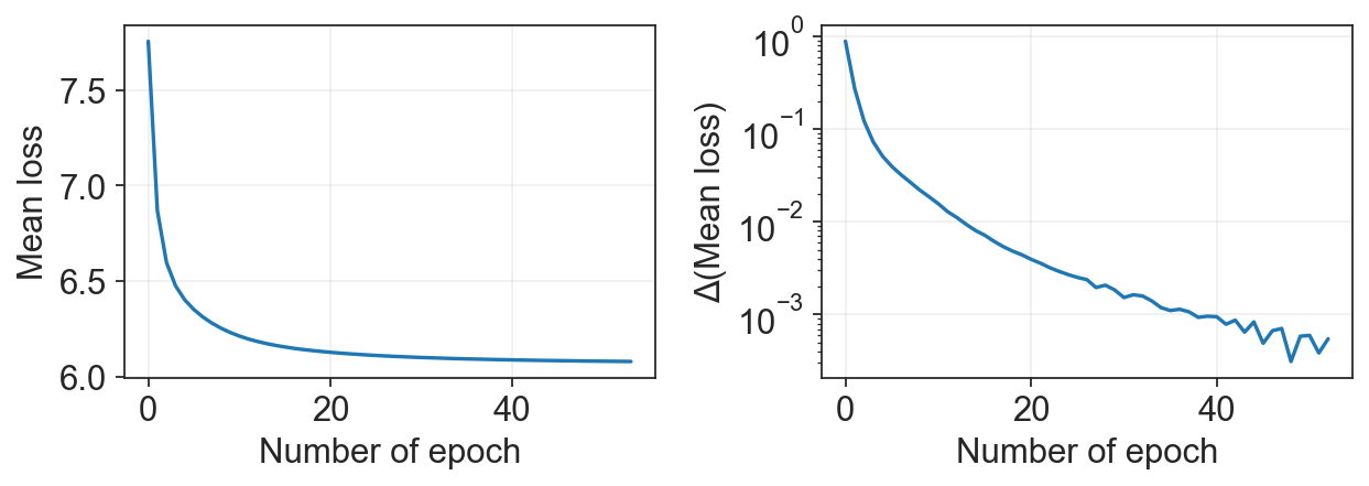
c2v.tl.clone2vec(clones)

fitting clone2vec embeddings
    SG epochs:  11%|█         | 53/500 [13:24<1:53:05, 15.18s/it, loss=6.0780, Δ=9.01e-05]
    early stopping at epoch 54
    finished (0:13:26): added
     .obsm['clone2vec'] embedding matrix.
     .uns['clone2vec'] training details.

We can make sure that the model converged:

[9]:

c2v.pl.loss_history(clones)

It’s better to perform the training on the GPU. With CPU, the training (especially for large dataset and low CPU number) can take hours. If your training takes too much time, we suggest using c2v.tl.clone2vec_Poi() function instead, as it gives comparable quality of the embedding.

Exploration#

Now, we have our clonal embedding in clones.obsm["clone2vec"]. Let’s visualize it with UMAP.

[10]:

sc.pp.neighbors(clones, use_rep="clone2vec")

computing neighbors
    finished: added to `.uns['neighbors']`
    `.obsp['distances']`, distances for each pair of neighbors
    `.obsp['connectivities']`, weighted adjacency matrix (0:00:03)

[11]:

sc.tl.umap(clones)

computing UMAP
    finished: added
    'X_umap', UMAP coordinates (adata.obsm)
    'umap', UMAP parameters (adata.uns) (0:00:11)

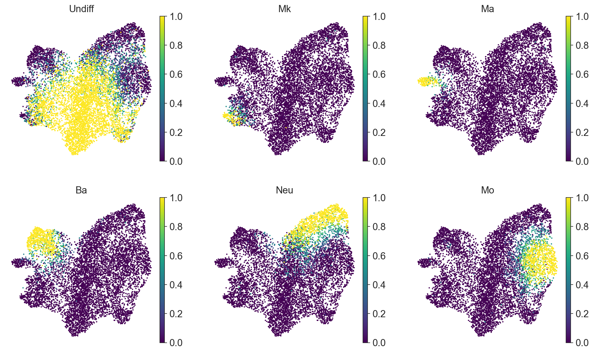
It can be convenient to plot a proportion of cell types per clone on this clonal UMAP.

[12]:

sc.pl.umap(
    clones,
    color=["Undiff", "Mk", "Ma", "Ba", "Neu", "Mo"],
    frameon=False,
    cmap="viridis",
    ncols=3,
)

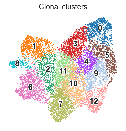
For the downstream analysis we can perform clustering via Leiden algorithm on clone2vec-derived kNN graph.

[13]:

sc.tl.leiden(
    clones,
    resolution=1,
    flavor="igraph",
    n_iterations=2,
)

running Leiden clustering
    finished: found 13 clusters and added
    'leiden', the cluster labels (adata.obs, categorical) (0:00:00)

[14]:

sc.pl.umap(
    clones,
    color="leiden",
    frameon=False,
    title="Clonal clusters",
    legend_loc="on data",
    legend_fontsize=15,
    legend_fontoutline=3
)

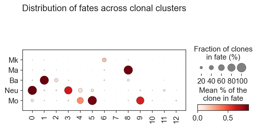
And we can visualize clusters’ composition via standart scanpy functions:

[15]:

sc.pl.dotplot(
    clones,
    var_names=["Mk", "Ma", "Ba", "Neu", "Mo"],
    groupby="leiden",
    colorbar_title="Mean % of the\nclone in fate",
    cmap="Reds",
    swap_axes=True,
    size_title="Fraction of clones\nin fate (%)",
    title="Distribution of fates across clonal clusters",
    dot_max=1,
)

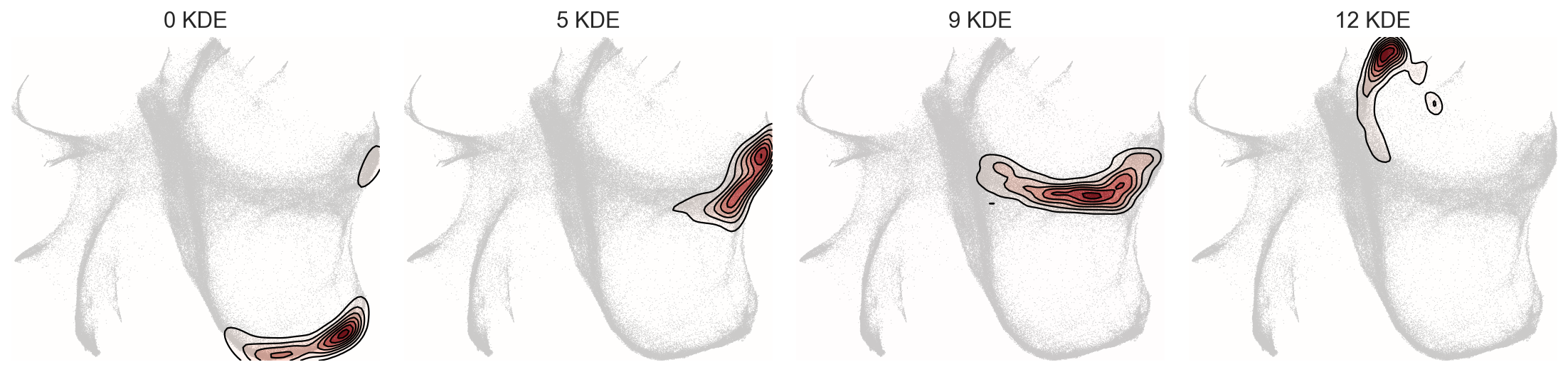
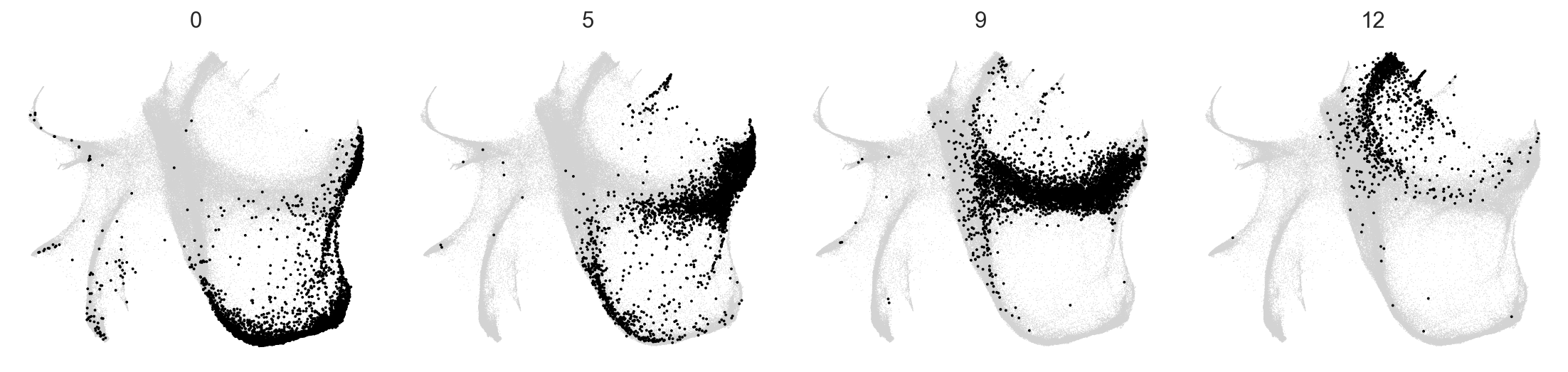
But the biggest advantage of clone2vec is that this algorithm makes possible to identify patterns of the distribution of clones without cell type information. Let’s check how cells from different clonal clusters look on the gene expression embedding.

[16]:

c2v.pp.transfer_annotation(adata, clones, annotation_obs_clones="leiden")

transferring annotations between cell and clone objects
    finished (0:00:00): added to clonal AnnData
     .obs['c2v_leiden'] categorical labels

After we transferred the annotation, let’s see how these distributions look like:

[17]:

selected_clusters = ["0", "5", "9", "12"]

c2v.pl.group_kde(adata, groupby="c2v_leiden", basis="X_spring", groups=selected_clusters)
c2v.pl.group_scatter(adata, groupby="c2v_leiden", basis="X_spring", groups=selected_clusters, s=12)

To explore these two embeddings, we can visualize them with c2v.pl.clones2cells() interactive widget (works in Jupyter or Google Colab — isn’t displayed in the html-version of tutorial):

[3]:

c2v.pl.clones2cells(
    adata=adata,
    clones=clones,
    cells_basis="X_spring",
    s_cells_bg=2,
    s_cells_selected=6,
    s_clones=8,
    height=450,
    cells_color="Cell type annotation short",
    keep_color=False,
    clones_color="leiden",
)

WARNING: Widget might be displayed incorrectly in Safari browser

Differences between wells and timepoints#

[31]:

c2v.pl.group_scatter(
    clones,
    groupby="gex_Time point",
    basis="X_umap",
    groups=[2, 4, 6],
    s=20,
    kwargs_group={
        "color": "gex_Time point",
        "legend_loc": None,
    },
)

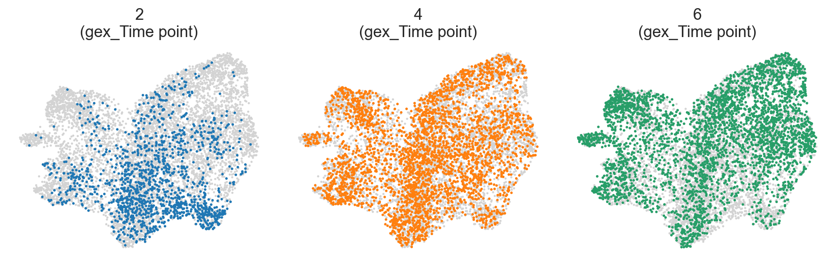
Question #1. Do wee see changes in clonal composition between timepoints at the same well?

[20]:

clones.obs["well:clone"] = (
    clones.obs["gex_Well"].astype(str) + ":" +
    clones.obs["gex_Clone"].astype(str)
)

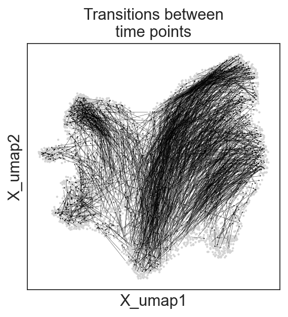
c2v.utils.connect_clones(clones, groupby="well:clone", orient_col="gex_Time point",
                        orient_rule="increase")

connecting clones:
    using .obs['well:clone'] to group clones
    finished (0:00:01): added
     .obsp['connected'] with graph of connected clones

[21]:

c2v.pl.graph(clones, graph_key="connected", oriented=True, linewidth=0.2,
            title="Transitions between\ntime points")

[22]:

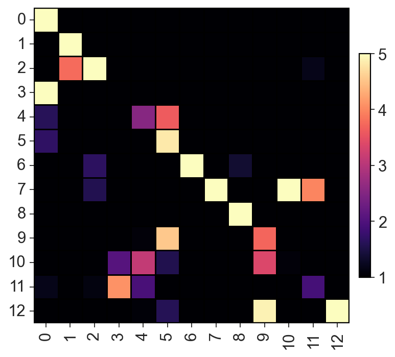
c2v.tl.group_connectivity(clones, groupby="leiden", graph_key="connected", directed=True)

computing groups connectivity matrix
    finished (0:00:00): added
     .uns['group_connectivity']['connectivity'] groups connectivity matrix
     .uns['group_connectivity']['label_names'] label names

[23]:

c2v.pl.heatmap(c2v.utils.get_connectivity_matrix(clones), vmin=1, vmax=5,
              cmap="magma", sort_columns=False)

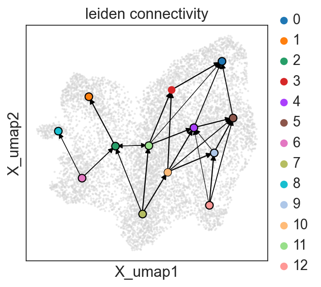
[24]:

c2v.pl.group_connectivity(clones, linewidth=0.5)

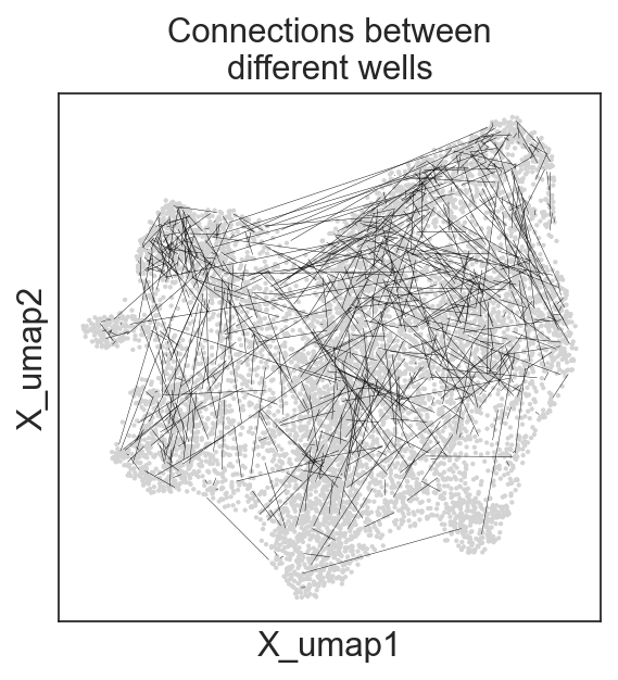
Question #2. Do we see changes in clonal composition between cells from the same time point, but different wells?

[25]:

clones.obs["time:clone"] = (
    clones.obs["gex_Time point"].astype(str) + ":" +
    clones.obs["gex_Clone"].astype(str)
)

c2v.utils.connect_clones(clones, groupby="time:clone")

connecting clones:
    using .obs['time:clone'] to group clones
    finished (0:00:00): added
     .obsp['connected'] with graph of connected clones

[26]:

c2v.pl.graph(clones, graph_key="connected", oriented=False, linewidth=0.2,
            title="Connections between\ndifferent wells")

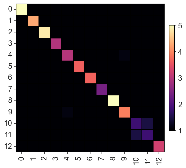
[27]:

c2v.tl.group_connectivity(clones, groupby="leiden", graph_key="connected", directed=False)

computing groups connectivity matrix
    finished (0:00:00): added
     .uns['group_connectivity']['connectivity'] groups connectivity matrix
     .uns['group_connectivity']['label_names'] label names

[28]:

c2v.pl.heatmap(c2v.utils.get_connectivity_matrix(clones), vmin=1, vmax=5,
              cmap="magma", sort_columns=False)

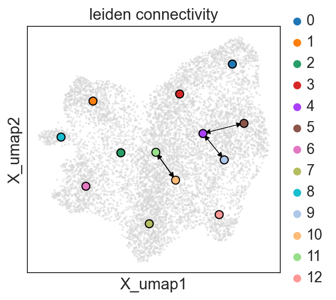
[29]:

c2v.pl.group_connectivity(clones, linewidth=0.5)

Also we can save our clonal AnnData to read later.

[30]:

clones.write_h5ad("Weinreb_clones.h5ad")
adata.write_h5ad("Weinreb_cells.h5ad")

Introduction to clonal embeddings

Contents

Introduction to clonal embeddings#

Preprocessing#

Clonal embedding#

Exploration#

Differences between wells and timepoints#