Fast clonal embeddings construction with py-fastglmpca#
In this notebook, we will build a clonal embedding with py-fastlmpca: quick alternative for the classical Skip-Gram approach.
The main difference with the classical clone2vec is that in the case of Poisson EPCA we can significantly simplify the calculation of the clonal embedding with the Alternating Poisson Regression approach (Weine et al., 2024), which we implemented in the `py-fastglmpca <serjisa/py-fastglmpca>`__ package with GPU support.
[1]:
import scanpy as sc
import numpy as np
import pandas as pd
import seaborn as sns
import matplotlib.pyplot as plt
import clone2vec as c2v

sc.set_figure_params(dpi=80)
sc.settings.verbosity = 3
sns.set_style("ticks")
Clonal embedding#
In this tutorial, we will read the clonal AnnData generated with the classical clone2vec and take the matrix of clonal neighbors in gene expression space from there.
[2]:
clones = sc.read_h5ad("Weinreb_clones.h5ad")
Instead of calling c2v.tl.clone2vec() function, we can call a wrapper around py-fastglmpca: c2v.tl.clone2vec_Poi().
[3]:
c2v.tl.clone2vec_Poi(clones)
fitting clone2vec_Poi embeddings
    GLM-PCA epochs:  17%|█▋        | 83/500 [01:22<06:55,  1.00it/s, Log-Likelihood=-1462331.5000, Δ=9.97e-05, LR=5.00e-01]
    finished (0:01:23): added
     .obsm['clone2vec_Poi'] embedding matrix.
     .uns['clone2vec_Poi'] training details.
[4]:
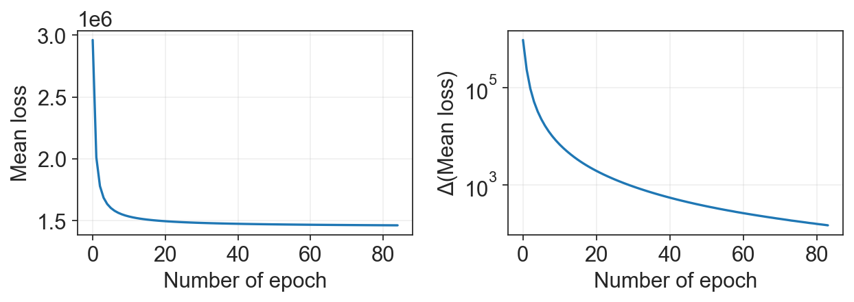
c2v.pl.loss_history(clones, uns_key="clone2vec_Poi")
Comparison of clonal embeddings#
We can head-to-head inspect our clonal embeddings (at least visually). To do that, let’s build a clustering and UMAP based on the new clonal embedding.
[5]:
sc.pp.neighbors(clones, use_rep="clone2vec_Poi", n_neighbors=15, key_added="Poi")
computing neighbors
    finished: added to `.uns['Poi']`
    `.obsp['Poi_distances']`, distances for each pair of neighbors
    `.obsp['Poi_connectivities']`, weighted adjacency matrix (0:00:08)
[6]:
sc.tl.umap(clones, neighbors_key="Poi", key_added="X_umap_Poi")
computing UMAP
    finished: added
    'X_umap_Poi', UMAP coordinates (adata.obsm)
    'X_umap_Poi', UMAP parameters (adata.uns) (0:00:11)
[7]:
sc.tl.leiden(clones, neighbors_key="Poi", key_added="leiden_Poi",
             flavor="igraph", n_iterations=2)
running Leiden clustering
    finished: found 13 clusters and added
    'leiden_Poi', the cluster labels (adata.obs, categorical) (0:00:00)
To visually inspect differences between embeddings, let’s plot a grid of both clusterings on both UMAPs.
[8]:
fig, axes = plt.subplots(ncols=2, nrows=2, figsize=(8, 8))

sc.pl.embedding(clones, basis="X_umap_Poi", ax=axes[0, 0], show=False, color="leiden_Poi", legend_loc="on data",
                legend_fontoutline=2, title="Poisson GLM-PCA clusters")
sc.pl.embedding(clones, basis="X_umap_Poi", ax=axes[0, 1], show=False, color="leiden", legend_loc="on data",
                legend_fontoutline=2, title="clone2vec clusters")

sc.pl.embedding(clones, basis="X_umap", ax=axes[1, 0], show=False, color="leiden_Poi", legend_loc="on data",
                legend_fontoutline=2, title="Poisson GLM-PCA clusters")
sc.pl.embedding(clones, basis="X_umap", ax=axes[1, 1], show=False, color="leiden", legend_loc="on data",
                legend_fontoutline=2, title="clone2vec clusters")
[8]:
<Axes: title={'center': 'clone2vec clusters'}, xlabel='X_umap1', ylabel='X_umap2'>
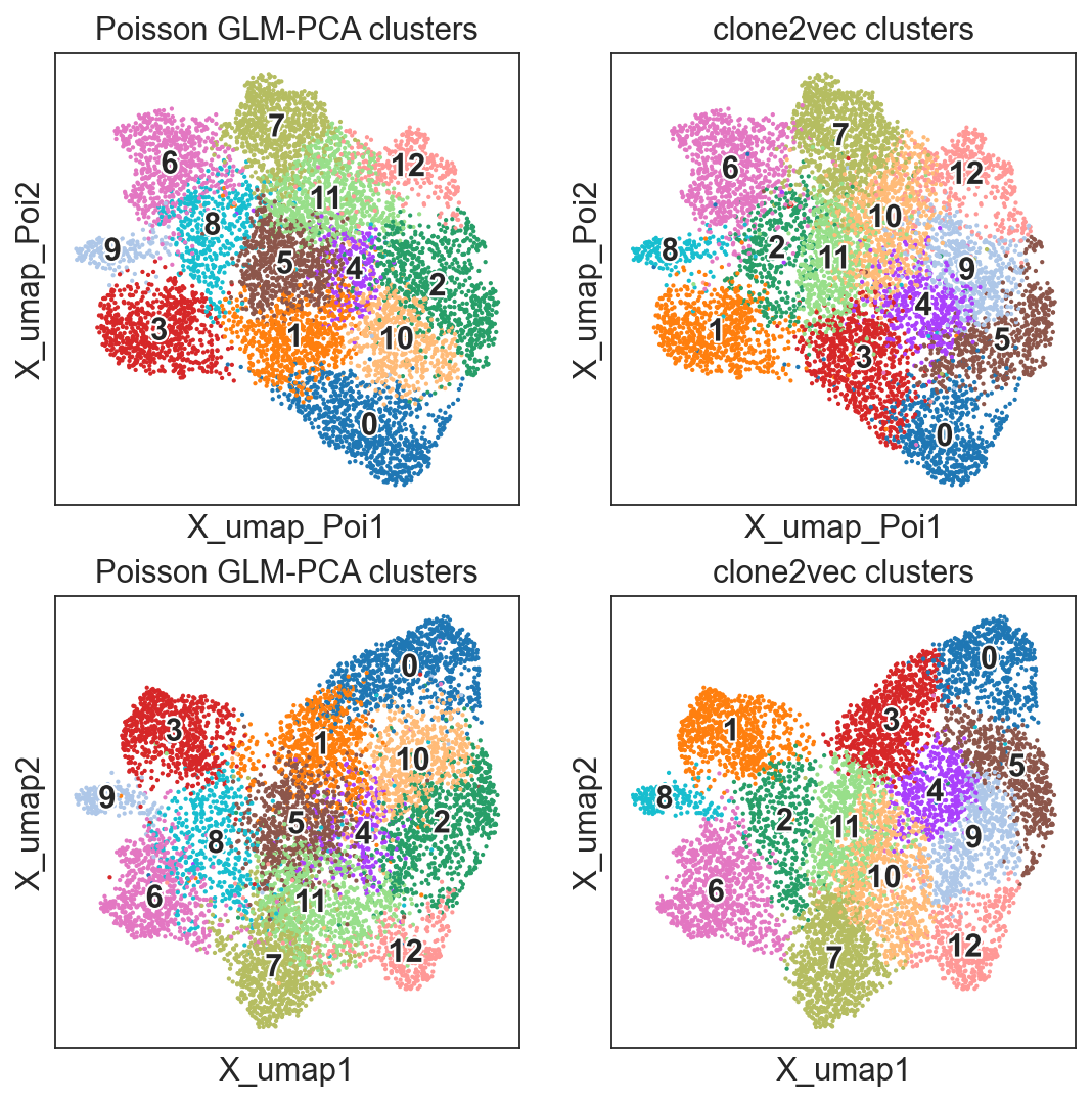
Now it looks a bit different (though clusters are pretty consistent between embeddings), but let’s flip UMAP of the GLM-PCA embedding:
[10]:
clones.obsm["X_umap_Poi_rotated"] = -clones.obsm["X_umap_Poi"].copy()
clones.obsm["X_umap_Poi_rotated"][:, 0] = -clones.obsm["X_umap_Poi_rotated"][:, 0]

fig, axes = plt.subplots(ncols=2, nrows=2, figsize=(8, 8))

sc.pl.embedding(clones, basis="X_umap_Poi_rotated", ax=axes[0, 0], show=False, color="leiden_Poi", legend_loc="on data",
                legend_fontoutline=2, title="Poisson GLM-PCA clusters")
sc.pl.embedding(clones, basis="X_umap_Poi_rotated", ax=axes[0, 1], show=False, color="leiden", legend_loc="on data",
                legend_fontoutline=2, title="clone2vec clusters")

sc.pl.embedding(clones, basis="X_umap", ax=axes[1, 0], show=False, color="leiden_Poi", legend_loc="on data",
                legend_fontoutline=2, title="Poisson GLM-PCA clusters")
sc.pl.embedding(clones, basis="X_umap", ax=axes[1, 1], show=False, color="leiden", legend_loc="on data",
                legend_fontoutline=2, title="clone2vec clusters")
[10]:
<Axes: title={'center': 'clone2vec clusters'}, xlabel='X_umap1', ylabel='X_umap2'>
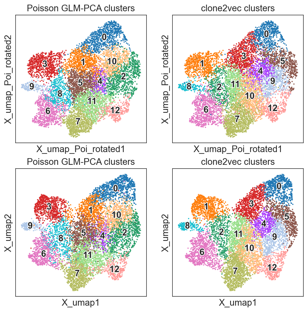
Now we see that even UMAPs look very similar.